Abstract

The objective of this study is to analyze the energy performance of two types of water-cooled air conditioning systems, variable air volume (VAV) and variable refrigerant flow (VRF), in terms of their cooling energy use through building simulation. These systems were designed to operate in an office building located in the city of Florianópolis, Brazil. The analysis involved the application of two building use schedules: a) constant and b) variable. Moreover, an analysis of the coefficient of performance (COP) and partial load ratio (PLR), and the percentage of operating hours for each range of cooling COP and PLR for each air conditioning system, allowed the system cooling efficiency to be assessed and the results to be related to the annual energy consumption. The coefficient of performance of VAV and VRF is 6.7 and 5.0, respectively, but the VRF system presented the lowest energy consumption for both schedules. The difference in the cooling energy consumption values for the VRF and VAV systems, for the variable schedule compared with the constant schedule, is mainly influenced by the partial load performance during the hottest period of the year.

Keywords:
Cooling Energy Performance; Building Energy Simulation; VAV; VRF

Resumo

O objetivo deste estudo é analisar o desempenho energético de dois tipos de sistemas de condicionamento de ar, volume de ar variável (VAV) e fluxo de refrigerante variável (VRF), com base no uso de energia em refrigeração através de simulação computacional. Os dois sistemas foram projetados para operar em um prédio comercial localizado na cidade de Florianópolis, Brasil. A análise envolveu a aplicação de dois padrões de uso da edificação: a) constante e b) variável. Além disso, o coeficiente de performance (COP), a razão de carga parcial (PLR), e o percentual anual de horas de operação para cada faixa de valores de COP e PLR para cada sistema de condicionamento de ar foram analisados, permitindo avaliar a eficiência de resfriamento do sistema e relacionar os resultados ao consumo anual de energia. O COP de entrada do VAV é 6.7 e do VRF é 5.0, mas o sistema VRF apresentou o menor consumo de energia para ambos padrões de uso. A diferença nos valores de consumo de energia de refrigeração para os sistemas VRF e VAV, para o padrão de uso variável comparado com o padrão de uso constante, é influenciada principalmente pelo desempenho da carga parcial durante o período mais quente do ano.

Palavras-chave:
Desempenho energético para refrigeração; Simulação computacional; VAV; VRF

Introduction

Energy efficiency currently represents a theme with major potential for research, mainly because of increased environmental and economic concerns and technological advances. In this regard, important achievements have been made in the area of buildings, due to their contribution to the total energy consumption, mostly associated with the air conditioning system, which accounts for a significant percentage of this consumption (ZHOU et al., 2008ZHOU, Y. P. et al. Simulation and experimental validation of the variable-refrigerant-volume (VRV) air-conditioning system in EnergyPlus. Energy and Buildings , v. 40, p. 1041-1047, 2008.; AYNUR; HWANG; RADERMACHER, 2009AYNUR, T. N.; HWANG, Y.; RADERMACHER, R. Simulation comparison of VAV and VRF air conditioning systems in an existing building for the cooling season. Energy and Buildings, v. 41, p. 1143-1150, 2009.). In 2018 IEA (International Energy Agency) has published the report “The Future of Cooling” that alerts us for the tremendous space cooling problem to come in future years. The energy use for space cooling is growing fast in the world and has tripled from 1990 to 2016 (INTERNATIONAL…, 2018INTERNATIONAL ENERGY AGENCY. The Future of Cooling. Paris: 2018.). This is putting an enormous strain on electricity systems in many countries and Brazil is one of them. We need firm policy interventions and more efficient air conditioners to minimize the effect on the electricity grid. An assessment of commercial offices in Brazil indicated that the air conditioning systems represent from 25% to 75% of the total energy consumption (GHISI; GOSCH; LAMBERTS, 2007GHISI, E.; GOSCH, S.; LAMBERTS, R. Electricity end-uses in the residential sector of Brazil. Energy Policy, v. 35, p. 4107-4120, 2007. ).

Many countries have developed and improved their energy labelling in buildings since the energy crisis in the 1970s, especially in the United States and Europe, where the economy is extremely dependent on oil. Investments in energy efficiency provide financial rewards and environmental benefits. However, in Brazil, efforts to introduce building regulations in this regard are more recent. The first energy efficiency law in Brazil was approved in 2001 (BRASIL, 2001BRASIL. Lei No. 10.295, de 17 de outubro de 2001, que dispõe sobre a Política Nacional de Conservação e Uso Racional de Energia e dá outras providências. Diário Oficial da República Federativa do Brasil, Brasília, 2001.). This resulted in an energy efficiency labelling system, the Regulation for Energy Efficiency Labelling of Commercial Buildings in Brazil (RTQ-C) (BRASIL, 2009BRASIL. Portaria no 53, de 27 de fevereiro de 2009, que regulamento Técnico da Qualidade do Nível de Eficiência Energética de Edifícios Comerciais, de Serviços e Públicos. Instituto Nacional de Metrologia, Normalização e Qualidade Industrial. Rio de Janeiro, 2009.), introduced in 2009. The RTQ-C classifies buildings according to five levels: from “A” (most efficient) to “E” (least efficient) according to the building envelope, lighting system and air conditioning system. This classification can be based on a surrogate model or obtained using building energy simulation programs. According to the surrogate model, the efficiency requirements for central air conditioning systems are based on standardized measurements under nominal conditions, such as coefficient of performance (COP) and integrated part load value (IPLV), according to ASHRAE Standard 90.1 minimum requirements (AMERICAN…, 2013aAMERICAN SOCIETY OF HEATING, REFRIGERATING AND AIR-CONDITIONING ENGINEERS. ANSI/ASHRAE Standard 90.1: energy standard for building except low-rise residential buildings. Atlanta, 2013a.). The simulation method consists of comparing two models: real/proposed and reference building. The two models must have common characteristics, such as same air conditioning system type and set point temperature. However, the real/proposed model should also adopt its own characteristics, for instance, for COP and IPLV. In Brazil, the energy efficiency of HVAC systems is measured according to ISO 5151 (INTERNATIONAL…, 2017INTERNATIONAL ORGANIZATION FOR STANDARDIZATION. ISO 5151: non-ducted air conditioners and heat pumps: testing and rating for performance. Geneva, 2017. ), where the equipment is evaluated under full load and under a standard temperature condition for heat absorption and rejection. However, there are no minimum efficiency standards for chillers, VRF (variable refrigerant flow) and self-contained air conditioning system. Therefore, the Brazilian regulation for non-residential buildings adopted the System Part Load Value (SPLV) to determine the efficiency of the system. SPLV is a single numerical indicator of part-load performance and a representative indication of a system performance operating under specific conditions. The SPLV calculation is based on the annual thermal load and the performance of the entire air=conditioning system, considering four thermal load conditions (100%, 75%, 50% and 25%). It is based on IPLV calculation methodology for equipment but covers all equipment involved in the air conditioning system and is calculated specifically for the project using actual weather data, actual part load characteristics, actual equipment performance, and the anticipated operating hours.

The variable air volume (VAV) air conditioning systems were introduced in the 1960s to reduce building energy consumption during operation at partial load (AYNUR; HWANG; RADERMACHER, 2009AYNUR, T. N.; HWANG, Y.; RADERMACHER, R. Simulation comparison of VAV and VRF air conditioning systems in an existing building for the cooling season. Energy and Buildings, v. 41, p. 1143-1150, 2009.) and have reached a consolidated acceptance on the market (YAO et al., 2007YAO, Y. et al. Evaluation program for the energy-saving of variable-air-volume systems. Energy and Buildings , v. 39, p. 558-568, 2007.; AYNUR, 2010AYNUR, T. N. Variable refrigerant flow systems: a review. Energy and Buildings, v. 42, p. 1106-1112, 2010.). This type of system has a lower acquisition cost compared to variable refrigerant flow (VRF) systems and presents flexibility and control in relation to the air distribution and design requirement (AYNUR; HWANG; RADERMACHER, 2008AYNUR, T. N., HWANG, Y.; RADERMACHER, R. The effect of the ventilation and the control mode on the performance of a VRF system in cooling and heating modes. In: INTERNATIONAL REFRIGERATION AND AIR CONDITIONING CONFERENCE, Purdue, 2008. Proceedings […] Purdue, 2008.; AYNUR, 2010AYNUR, T. N. Variable refrigerant flow systems: a review. Energy and Buildings, v. 42, p. 1106-1112, 2010.). The VAV air conditioning system consists of modulating the motor rotation of the blower fan through a frequency inverter in order to provide the necessary airflow to each conditioned zone according to its demand for thermal load. One of the other main benefits of typical VAV systems is the ability to use airside economizing to provide cooling when outside conditions are favorable. Thus, the reduction in the energy consumption, in relation to systems with constant air volume, is related with the blower fan and due to a reduction in the airflow that passes through the coil to be cooled. This affects the chiller performance, which is the most important factor in terms of the system energy consumption.

Centrifugal chillers are commonly adopted in large buildings, as their capacity is a function of the amount of refrigerant to be displaced and operation. According to ASHRAE (AMERICAN…, 2012AMERICAN SOCIETY OF HEATING, REFRIGERATING AND AIR-CONDITIONING ENGINEERS. ANSI/ASHRAE HVAC Systems and Equipment. Atlanta, 2012.), the capacity control in a centrifugal compressor is mainly performed in two ways: using a pre-rotation at the inlet rotor (known as pre-rotation vanes or inlet guide vanes) or variable speed drive (VSD). In the pre-rotation, fins installed in the suction of the rotor are operated by an electric-pneumatic mechanism, in order to regulate the flow of refrigerant according to a signal coming from a sensor that controls the chilled water temperature. In the case of VSD, the compressor capacity is controlled by varying the rotation speed of the rotor, the flow of refrigerant in the suction and the pressure in the discharge of the compressor.

In the search for increased energy efficiency in buildings and their systems, air conditioning system companies have been improving the variable refrigerant flow (VRF) technology (AYNUR; HWANG; RADERMACHER, 2009AYNUR, T. N.; HWANG, Y.; RADERMACHER, R. Simulation comparison of VAV and VRF air conditioning systems in an existing building for the cooling season. Energy and Buildings, v. 41, p. 1143-1150, 2009.; LI; WU; SHIOCHI, 2009LI, Y.; WU, J.; SHIOCHI, S. Modeling and energy simulation of the variable refrigerant flow air conditioning system with water-cooled condenser under cooling conditions. Energy and Buildings, v. 41, p. 949-957, 2009.; LI, WU, 2010LI, Y.; WU, J. Energy simulation and analysis of the heat recovery variable refrigerant flow system in winter. Energy and Buildings, v. 42, p. 1093-1099, 2010.). The VRF air conditioning system was introduced in Japan in the early 1980s. It is a central multi-split direct expansion system that varies the refrigerant flow according to the use of a variable speed compressor and to the electronic expansion valves (EEVs) situated in each indoor unit, which connects to the outdoor unit through the same refrigeration circuit. There are three different types of VRF available on the market today: single cold type, heat pump type and heat recovery type. The heat pump VRF system only supplies cooling or heating at a time and the heat recovery VRF system supplies both cooling and heating simultaneously. The outdoor unit can be air-cooled or water-cooled; and the main type of compressor used is the scroll. The main advantages of using the VRF system are a flexible and compact configuration, easy operation, individualized comfort control, and a high coefficient of performance in the partial load condition compared to other central air conditioning systems (AMARNATH, BLATT, 2008AMARNATH, A.; BLATT, M. Variable Refrigerant flow: an emerging air conditioner and heat pump technology. In: ACEEE SUMMER STUDY ON ENERGY EFFICIENCY IN BUILDINGS, Pacific Grove, 2008. Proceedings […] Pacific Grove, 2008.). This technology is becoming more frequently adopted in office buildings in Brazil. The competition in this segment is increasing around the world due to a strong commercial appeal focused on sustainability and energy saving (LI, WU, 2010LI, Y.; WU, J. Energy simulation and analysis of the heat recovery variable refrigerant flow system in winter. Energy and Buildings, v. 42, p. 1093-1099, 2010.; LIU, WONG, 2010LIU, X.; HONG, T. Comparison of energy efficiency between variable refrigerant flow systems and ground source heat pump systems. Energy and Buildings, v. 42, p. 584-589, 2010.). The various benefits of VRF systems drive the growth in the market of this system globally. In Asia and Europe, the VRF air conditioning system is well accepted in the market. In Japan, the VRF system has been used in approximately 50% of medium-sized commercial buildings and in 33% of large buildings. In Europe, where many existing buildings do not have air conditioning, retrofit opportunities represent a growing demand for their application. In the US, although the VRF air-conditioning market is still growing, Asian manufacturers seek a position, individually or in partnership with US manufacturers (AMARNATH, BLATT, 2008AMARNATH, A.; BLATT, M. Variable Refrigerant flow: an emerging air conditioner and heat pump technology. In: ACEEE SUMMER STUDY ON ENERGY EFFICIENCY IN BUILDINGS, Pacific Grove, 2008. Proceedings […] Pacific Grove, 2008.).

The improvement of building energy simulation programs, especially in the last decade, has provided support in studies on air conditioning system efficiency. Computational simulations represent a significant collaboration in the context of sustainable development, supporting building labeling programs, especially in Brazil, where investments in this regard are recent. Also, building energy simulation allows technical and economic analysis of the cost/benefit ratio to be carried out during the design process.

Literature review

Comparative studies regarding VRF system performance are recent. VRF models have been developed and implemented in DOE-2.1E and IES-VE (HONG et al., 2016HONG, T. et al. Development and validation of a new variable refrigerant flow system model in EnergyPlus. Energy and Building, v. 117, p. 399-411, 2016.) and available in Trace700, eQuest, EnergyPro and EnergyPlus (AMARNATH, BLATT, 2008AMARNATH, A.; BLATT, M. Variable Refrigerant flow: an emerging air conditioner and heat pump technology. In: ACEEE SUMMER STUDY ON ENERGY EFFICIENCY IN BUILDINGS, Pacific Grove, 2008. Proceedings […] Pacific Grove, 2008.). Studies to improve the VRF simulation in EnergyPlus program have been conducted since 2007, considering several configurations: air cooled VRF systems (ZHOU et al., 2007ZHOU, Y. P. et al. Energy simulation in the variable refrigerant flow air-conditioning system under cooling conditions. Energy and Buildings , v. 39, p. 212-220, 2007.), water-cooled VRF systems (LI, WU, 2010LI, Y.; WU, J. Energy simulation and analysis of the heat recovery variable refrigerant flow system in winter. Energy and Buildings, v. 42, p. 1093-1099, 2010.) and heat recovery VRF systems (AMARNATH, BLATT, 2008AMARNATH, A.; BLATT, M. Variable Refrigerant flow: an emerging air conditioner and heat pump technology. In: ACEEE SUMMER STUDY ON ENERGY EFFICIENCY IN BUILDINGS, Pacific Grove, 2008. Proceedings […] Pacific Grove, 2008.).

Field research has also been conducted to evaluate the use of these implementations (ZHOU et al., 2008ZHOU, Y. P. et al. Simulation and experimental validation of the variable-refrigerant-volume (VRV) air-conditioning system in EnergyPlus. Energy and Buildings , v. 40, p. 1041-1047, 2008.; LI et al., 2010LI, Y.; WU, J. Energy simulation and analysis of the heat recovery variable refrigerant flow system in winter. Energy and Buildings, v. 42, p. 1093-1099, 2010.; EGAN, 2009EGAN, A. M. three case studies using building simulation to predict energy performance of 16 Australian office buildings. In: IBPSA BUILDING SIMULATION CONFERENCE, Glasgow, 2009. Proceedings […] Glasgow, 2009.). The EnergyPlus program, version 7.2 (ENERGYPLUS, 2018ENERGYPLUS. EnergyPlus program. Disponível em: https://energyplus.net. Acesso em: 3 mar. 2018.
https://energyplus.net... ), presented the first validated approach to modeling a VRF system, the System Curve-based Model (VRF-SysCurve) (RAUSTAD, 2013RAUSTAD, R. A variable refrigerant flow heat pump computer model in Energyplus, ASHRAE Transaction, v. 19, p. 299-308, 2013.). The validated VRF model was experimentally analyzed by Kim et al. (2018)KIM, D. et al. Model calibration of a variable refrigerant flow system with a dedicated outdoor air system: a case study. Energy and Building, v. 158, p. 884-896, 2018. and observed greater agreement between measured and simulated results when compared with results obtained by Zhou et al. (2008)ZHOU, Y. P. et al. Simulation and experimental validation of the variable-refrigerant-volume (VRV) air-conditioning system in EnergyPlus. Energy and Buildings , v. 40, p. 1041-1047, 2008.. In version 8.4, the EnergyPlus program presented a second VRF model named the Physics-based Model (VRF-FluidTCtrl), which was validated by Hong et al. (2016)HONG, T. et al. Development and validation of a new variable refrigerant flow system model in EnergyPlus. Energy and Building, v. 117, p. 399-411, 2016..

Studies indicate that the VRF system is becoming competitive in relation to the VAV chilled water system regarding the former potential reduction in energy consumption and higher partial load efficiency. Zhou et al. (2007)ZHOU, Y. P. et al. Energy simulation in the variable refrigerant flow air-conditioning system under cooling conditions. Energy and Buildings , v. 39, p. 212-220, 2007. simulated a 10-story office building in Shanghai and the air-cooled VRF systems could consume from 11% to 22% less energy compared to water-cooled chiller-based fan-coil plus fresh air systems (FPFA) and VAV systems, respectively. It was observed the air conditioning systems operated for around 80% of the time in a PLR range of 30% to 90%. The same building was analyzed by Li et al. (2009)LI, Q. et al. Predicting hourly cooling load in the building: a comparison of support vector machine and different artificial neural networks. Energy Conversion and Management, v. 50, p. 90-96, 2009. and the energy consumption of the VRF air-cooled system was 4% lower than the VRF water-cooled system and 24% lower than the fan-coil plus fresh air systems (FPFA). The greatest difference in cooling energy consumption was in June, when the PLR range was 0.35 to 0.6, and in July and August, when the PLR differ from 0.5 to 0.9. The energy savings of a VRF system compared to a VAV system was observed by Aynur, Hwang and Radermacher (2009)AYNUR, T. N.; HWANG, Y.; RADERMACHER, R. Simulation comparison of VAV and VRF air conditioning systems in an existing building for the cooling season. Energy and Buildings, v. 41, p. 1143-1150, 2009., in three different existing office building in Maryland, USA. Results show that VRF system ranged from 27.1% to 57.9% in relation to a central VAV systems, depending on the system configuration and design conditions. Yu et al. (2016)YU, X. et al. Comparative study of the cooling energy performance of variable refrigerant flow systems and variable air volume systems in office buildings. Applied Energy, v. 183, p. 725-736, 2016. compared the cooling energy use data for VAV and VRF systems in five typical office buildings in China, using a site survey and field measurements to quantify the impact of the system operation. The cooling energy savings of the VRF system was higher when compared to VAV system. Kim et al. (2017)KIM, D. et al. Evaluation of energy savings Potential of Variable Refrigerant flow (VRF) from Variable Air Volume (VAV) in the U.S. climate locations. Energy Reports, v. 3, p. 85-93, 2017. observed the energy saving potential of a VRF system in relation to a VAV system for 16 United States climates zones. It was observed that VRF saves more energy than a VAV system, and the amount depends on the climate zone. In general, energy savings in hot and mild climates are higher than in cold climates due to the heating energy consumption. These mentioned studies have set an acceptable system design Combination Ratio (CR) for their VRF system equipment. The CR is defined as the ratio of the capacity of the indoor units to the capacity of the outdoor unit coupled to them, and CR ranges vary from manufacturer to manufacturer. However, it is important to highlight the advantages and disadvantages by considering a larger or smaller CR.

The VAV chilled water and VRF air conditioning systems are adopted in energy efficient buildings in Brazil. However, simulation studies on both systems are still scarce in Brazil and in other countries, specifically those addressing the water-cooled VRF system. The Brazilian regulation for energy efficient buildings is in continuous development, not only to include updates regarding new technologies, but also to improve the efficiency level of the systems. Studies to address the performance of air conditioning systems can provide information that promotes the energy efficient use of buildings, either through stimulating new research or the adoption of better design practices.

This current study compares the VAV and VRF energy consumption and performance under nominal conditions and partial loads, addressing the importance of gaining information from the use of building energy simulation tools that allow air conditioning systems to be modelled, and the great contribution that these assessments can provide with regard to reducing building energy consumption. Moreover, the study intends to observe how the performance indexes, such as COP and IPLV, influence the energy efficiency of VAV and VRF systems in buildings.

Method

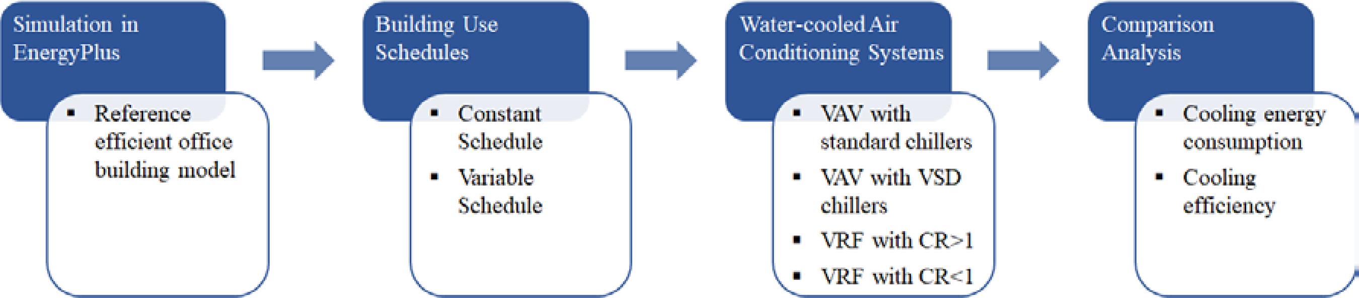
The comparative energy analysis methodology regarding the VAV (variable air volume) system and the VRF (variable refrigerant flow) system is presented in Figure 1. The VAV and VRF systems were simulated for an office building located in Florianópolis, Brazil, assuming the design practices and energy efficiency levels determined by the Brazilian Regulation for Energy Efficient Buildings. The computational simulations were run using the EnergyPlus program, version 8.1 to compare and analyze the energy performance of air conditioning systems. Two building use schedules, during the occupation period, were simulated: constant internal loads; and variable internal load to assess the use schedules performance on the energy consumption of VAV and VRF systems. The air conditioning system selection criteria and building energy simulation input data may radically alter the findings. However, the approach is a case study. The main focus is to assess results based on nominal projects requirements considered as efficient in the annual energy performance of air conditioning systems. Both air conditioning systems are water-cooled and single cold type and operate for cooling throughout the year. Each system is simulated with two configurations: VAV system with a centrifugal chiller with an inlet guide vanes-type compressor, named standard chiller, and a VSD centrifugal chiller; VRF system with combination ratio (CR) greater than 1 (CR > 1) and smaller than 1 (CR < 1). The performance curves for the chillers and outdoor VRF units are modeled considering manufacturer performance data, showing the differences of a system with a combination ratio greater or smaller than 1. The total cooling energy consumption from both air conditioning system is compared, and a discussion on the annual results according to the percentage of operation time for different COP and PLR values and the cooling energy performance is provided.

Design parameters of the air conditioning systems

The design days are very important for use in HVAC Sizing Calculation in EnergyPlus program, allowing the user to use a pre-defined design day profile based on ASHRAE Handbook of Fundamentals, or to create your own profile. For this study, the VAV and VRF systems cooling capacity were auto-sized based on a summer design day pre-defined according to ASHRAE Handbook of Fundamentals (AMERICAN…, 2013bAMERICAN SOCIETY OF HEATING, REFRIGERATING AND AIR-CONDITIONING ENGINEERS. ANSI/ASHRAE Hanbook Fundamentals. Atlanta, 2013b.) with sizing factor 1.15. The heating system was not considered in the simulations as it is not typical for office buildings in this location.

Performance curves were applied to determine VAV and VRF characteristics, being aware that a slight change in the performance curves would reflect on results. The same attention was also considered for all input data regarding the information from air conditioning system adopted. The decision about each system is based on three criteria:

1. 1. Capacity result dimensioned by the program;

2. 2. Availability of data from a real system; and

3. 3. Minimal requirements according to the Brazilian regulation for commercial buildings.

For cooling performance results, the influential inputs data are nominal capacity, COP and curves. Curves correct the available capacity and the power consumed during operation, with a value of 1 at a nominal condition. Varying the equipment capacity, influence the calculated PLR at each moment, affecting the consumption based on the nominal power. Varying the COP, influence the reference nominal power. For the main purpose in this case study, both VAV systems have the same input data and two curves of two different compressors are adopted. The VRF systems have same curves and same COP, but different nominal capacities. In addition, the COP value from VAV systems is different from VRF system.

Variable air volume system

Figure 2 provides a schematic diagram of the chilled water system. A conventional primary (constant)/secondary (variable) system was adopted. The chilled water load distribution scheme is sequential; the main chiller operates primarily, and the secondary chiller operates to complete the need for the cooling demand. The chilled water setpoint ranges from 6.7 ºC to 12 ºC when the outdoor air dry-bulb temperature ranges from 27ºC to 16ºC, and when this temperature is greater than 27ºC the setpoint is 6.7 ºC, and for lower than 16ºC the setpoint is 12 ºC. The condenser water setpoint changes according to the outdoor air wet-bulb temperature (plus 5.6 ºC).

The VAV air loop system is shown in Figure 3. All requirements and design considerations were identical for both VAV air conditioning systems considered, with centrifugal chillers and with VSD centrifugal chillers. All pumps have intermittent operation and shut off when no load is identified. The nominal power values adopted were 349 kW/m³/s for the chilled water pumps and 310 kW/m³/s for the condenser water pumps (AMERICAN…, 2012AMERICAN SOCIETY OF HEATING, REFRIGERATING AND AIR-CONDITIONING ENGINEERS. ANSI/ASHRAE HVAC Systems and Equipment. Atlanta, 2012.). The curve used for variable-speed pump power correction was selected from the DataSets folder of the EnergyPlus program, according to Equation 1.

Where:

• FFLPower is the fraction of full load power of the variable-speed pump;

• v is the current variable-speed pump water flow rate (m³/s); and

• v_designis the design maximum variable-speed pump water flow rate (m³/s).

The VAV supply fan has an efficiency of 0.65, pressure rise of 600 Pa and motor efficiency of 0.8. The curve for the fan power correction is modeled according to Appendix G of ASHRAE Standard 90.1 (AMERICAN…, 2013aAMERICAN SOCIETY OF HEATING, REFRIGERATING AND AIR-CONDITIONING ENGINEERS. ANSI/ASHRAE Standard 90.1: energy standard for building except low-rise residential buildings. Atlanta, 2013a.). The main VAV air conditioning systems are detailed in Table 1.

Three performance curves are applied to determine the chiller operation, to determine the COP and IPLV value (6.1 W/W and 6.4 W/W, respectively), and to adjust the available cooling capacity and energy consumption, according to Equations 2, 3 and 4:

Where:

• ChillerCapFTemp is the cooling capacity factor function of temperature;

• ChillerEIRFTemp is the energy input to cooling output factor function of temperature;

• ChillerEIRFPLR is energy input to cooling output factor function of PLR;

• T_cw,l is the leaving chilled water temperature (ºC);

• T_cond,e is the entering condenser water temperature (ºC);

• PLR is the partial-load ratio, cooling load/chiller available cooling capacity; and

• a to f are the coefficients of the performance curves.

In Brazil, the chiller performance curves are not commonly available by the manufactures. Therefore, the coefficients of performance curves for the standard and VSD centrifugal chillers adopted in the simulations were obtained from the DataSet folder of the EnergyPlus program: standard chiller Trane CVHE model with a capacity of 1329.3 kW and refrigerant fluid R-123 with a COP of 5.38 W/W and the VSD chiller Carrier 19XR model with a capacity of 1407 kW and refrigerant fluid R-134 with a COP of 6.04. All of the coefficient of performance curves values is presented in the Appendices A - Variable air volume system characteristics.

Variable refrigerant flow system

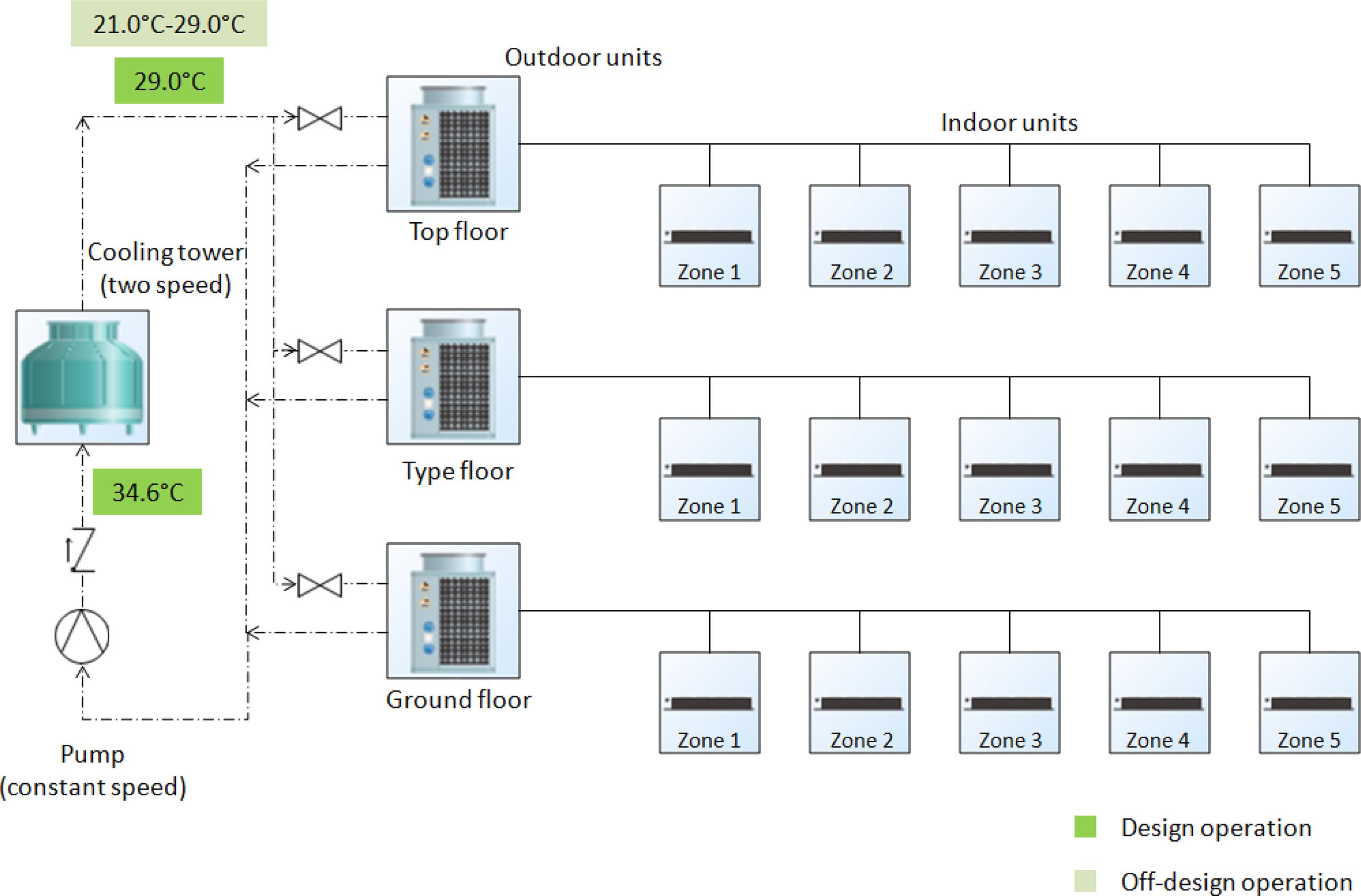
The indoor units of each thermal zone, represented by a single object for modeling purposes, are connected to an outdoor unit, that is a total of 15 subsystems, as shown in Figure 4. All design requirements and considerations are identical for the two VRF air conditioning systems, with the exception of the combination ratio (CR) selection for the outdoor units: with combination ratio (CR) greater than 1 (CR > 1) and smaller than 1 (CR < 1), highlighting the advantages and disadvantages by considering a larger or smaller CR.

Manufacturer catalogs (LG ELECTRONICS, 2014aLG ELECTRONICS. Air conditioner engineering product data book, multi V Water II, R410. 2014a. Disponível em: https://www.manualslib.com/products/Lg-Arwn480da2-3667303.html. Acesso em: 15 abr. 2018.
https://www.manualslib.com/products/Lg-A... ) were used to select the VRF equipment and modelling the characteristics, detailed in the Appendices B - Variable refrigerant flow system characteristics. The efficiency of indoor unit’s supply air fan is 0.65 and motor efficiency is 0.8. The air flow rate of the fan is constant and the supply fan operates continuously. The supply fan stays off when the VRF system is not demanded.

Two different outdoor unit models were selected for these indoor units to understand the differences of a system with a combination ratio greater or smaller than 1. The CR is a parameter chosen by the designer and, in addition to safety criteria, the choice is influenced by the cost/benefit ratio, the cost of the system per kW and the characteristic of better performance in partial load of the VRF system. The LG ARWN480DA2 outdoor unit was selected for the VRF system with a CR > 1, and the LG ARWN580DA2 outdoor unit for the VRF system with a CR < 1. The condenser water flow rate was adopted according to the catalog (LG ELECTRONICS, 2014bLG ELECTRONICS. Total HVAC Solution provider engineering product data book, multi V indoor unit, R410 A. 2014b. Disponível em: file:///C:/Users/user/Downloads/VRF-EM-BH-002-US-014A15_LGEngineeringManual_MultiVSpace_20140116144102.pdf.Acesso em: 15 abr. 2018.
file:///C:/Users/user/Downloads/VRF-EM-B... ). The other design and operating criteria for the condenser loop are the same as those used to configure the VAV air conditioning system. Data regarding the dimensional parameters adopted for the outdoor units, the condenser water pumps and the cooling tower of the VRF air conditioning systems are also given in the Appendices B - Variable refrigerant flow system characteristics

The EnergyPlus simulation model used was the VRF System Curve-based Model. The correction factors adjust the off-reference performance of the VRF system. In this study, the coefficients of the performance curves were obtained by polynomial regression using performance data obtained from catalogs (LG ELECTRONICS, 2014bLG ELECTRONICS. Total HVAC Solution provider engineering product data book, multi V indoor unit, R410 A. 2014b. Disponível em: file:///C:/Users/user/Downloads/VRF-EM-BH-002-US-014A15_LGEngineeringManual_MultiVSpace_20140116144102.pdf.Acesso em: 15 abr. 2018.
file:///C:/Users/user/Downloads/VRF-EM-B... ).

Two curves were fitted to the available cooling capacity of the indoor unit, according to Equations 5 and 6:

Where:

• TotCapTempModFac is the total capacity modifier curve function of temperature;

• TotCapFlowModFac is the total capacity modifier curve function of flow fraction;

• T_wb,i is the wet-bulb temperature of the air entering the cooling coil (ºC);

• ff is the flow fraction, actual air flow rate/rated air flow rate; and

• a to b are the coefficients of performance curves.

The same coefficients of performance were adopted for the curves related to all indoor units. The model used as a reference was the LG ARNU423BGA2 (LG ELECTRONICS, 2014bLG ELECTRONICS. Total HVAC Solution provider engineering product data book, multi V indoor unit, R410 A. 2014b. Disponível em: file:///C:/Users/user/Downloads/VRF-EM-BH-002-US-014A15_LGEngineeringManual_MultiVSpace_20140116144102.pdf.Acesso em: 15 abr. 2018.
file:///C:/Users/user/Downloads/VRF-EM-B... ). The coefficients of performance curves are reported in the Appendices B - Variable refrigerant flow system characteristics. For each indoor unit, the cooling capacity data, as a function of the wet-bulb temperature obtained from the catalogs is compared with the cooling capacity calculated using the TotCapFlowModFac curve obtained from LG ARNU423BGA2 (Figure 5). It was observed the difference was not relevant.

Eleven curves were fitted to the available cooling capacity and electricity consumption of the outdoor unit, according to Equations 7 to 17:

Where:

• CAPFT_low is the capacity ratio modifier function of low temperature;

• CAPFT_high is the capacity ratio modifier function of high temperature;

• T_cond,capft is the capacity ratio boundary, entering condenser water temperature boundary;

• EIRFT_low is the energy input ratio modifier function of low temperature;

• EIRFT_high is the energy input ratio modifier function of high temperature;

• T_cond,EIRft is the energy input ratio boundary, entering condenser water temperature boundary;

• EIRFPLR_high is the energy input ratio modifier function of high part-load ratio, PLR>1;

• EIRFPLR_low is the energy input ratio modifier function of low part-load ratio, PLR≤1;

• CR_correction is the combination ratio capacity correction factor;

• P_correction is the piping correction factor for length;

• PLF is the part-load fraction correlation, factor is used to account for startup losses of the compression system, when it cycles on and off. The default value of the EnergyPlus program was adopted as the data for this curve is not reported in catalogs;

• T_wb,avg is the load-weighted average wet-bulb temperature of the air entering all operating cooling coils (ºC);

• T_cond,e is the entering condenser water temperature (ºC);

• PLR is the partial-load ratio, actual cooling capacity / available cooling capacity;

• CR_rated is the combination ratio, rated total cooling capacity of the indoor terminal unit divided by the rated total cooling capacity of outdoor terminal unit;

• P_EQ is the equivalent piping length between indoor terminal unit and outdoor terminal unit (m);

• P_H is the vertical height between indoor terminal unit and outdoor terminal unit (m);

• PLR_min is the minimum partial-load ratio; and

• a to f are the coefficients of performance curves.

Schedule for air conditioning system

Two different building use schedules were adopted. The first one is a constant schedule (Table 2), often considered for the evaluation of office building energy performance, in Brazil, when no database for the building use is available. The constant schedule was adopted to size the cooling system. The second is a variable schedule (Table 3), based on the office occupancy described by ASHRAE (AMERICAN…, 2007AMERICAN SOCIETY OF HEATING, REFRIGERATING AND AIR-CONDITIONING ENGINEERS. ANSI/ASHRAE Standard 90.1 User’s Manual: energy standard for building except low-rise residential buildings. Atlanta, 2007.), modified to match the working hours in Brazil. As the cooling energy demand should be lower for a variable schedule, it is important to observe the performance of the air conditioning systems in partial load operation for different cooling demands.

The zone thermostat setpoint was 24ºC for both types of air conditioning systems, from 08:00 to 20:00 on weekdays and from 08:00 to 12:00 on Saturdays. For Sundays and public holidays, the air conditioning system is off. Any optimal automation system was considered for the air conditioning system.

The prototype building model

The building model has 15 floors, each with 30 m x 30 m x 3 m (Figure 6), with five thermal zones, 4.5 m room depth (one central and four peripherals) recommended by ASHRAE (AMERICAN…, 2013).

The envelope thermal transmittance constructive system is based on requirements established in the Regulation for Energy Efficiency Labelling of Office Buildings in Brazil (BRASIL, 2009BRASIL. Portaria no 53, de 27 de fevereiro de 2009, que regulamento Técnico da Qualidade do Nível de Eficiência Energética de Edifícios Comerciais, de Serviços e Públicos. Instituto Nacional de Metrologia, Normalização e Qualidade Industrial. Rio de Janeiro, 2009.) in accord with Table 4, with 50% window to wall ratio, green glass 6 mm thick, 0.623 solar factor. The solar absorptance is 0.5 for walls and roof.

The internal loads parameters are also based on requirements established in the Regulation for Energy Efficiency Labelling of Commercial Buildings in Brazil (BRAZIL, 2009), represented by equipment (155 W/person), lighting (9.7 W/m²), and people (7 m²/person).

The air conditioning air change rate was a constant rate of 27 m³/h.person, considering a nominal occupancy rate for the entire period. The thermal zones were considered slightly pressurized during the operation of the air conditioning system. During the period of non-operation of the air conditioning system, an air infiltration rate of 0.5 air change per hour (ACH) was adopted for all thermal zones.

The weather data type assumed is a Test Reference Year (TRY) for the city of Florianópolis. According to NBR - 15220-3: Thermal performance of buildings (ABNT, 2005ASSOCIAÇÃO BRASILEIRA DE NORMAS TÉCNICAS. NBR 15220: desempenho térmico de edificações: parte 2: métodos de cálculo da transmitância térmica, da capacidade térmica, do atraso térmico e do fator solar de elementos e componenentes de edificações. Rio de Janeiro, 2005. ), the city of Florianópolis is in Zone 03. Considering Koppen’s climate classification, Florianópolis is defined as a Humid Subtropical Climate. The number of cooling degree hours (24ºC) is 4517 (GOULART, 1993GOULART, S. V. G. Dados Climáticos para avaliação de desempenho térmico em Florianópolis. Florianópolis, 1993. Tese (Doutorado em Engenharia Civil) - Escola de Engenharia, Universidade Federal de Santa Catarina, Florianópolis, 1993. ).

Cooling energy analysis

The cooling loads of the VRF and VAV systems were compared, according to two building use schedules (constant and variable). The end use energy consumption represents the importance of cooling, fan, tower and pumps for both systems, including impact on partial load.

The annual energy consumption and performance under nominal conditions and partial loads was also performed for VAV and VRF systems. Therefore, the percentage of hours for which the systems operated in each range of COP and PLR values was investigated, to assess the achievement of the design concepts used as parameters of efficient choices for the systems applied in the case study.

Results

Performance curves

Variable air volume system

The standard chiller nominal COP was 6.7 W/W, resulting in a COP of 6.51 W/W and an IPLV of 6.41 for the current the design operation. For the VSD chiller, the nominal COP modeled was also 6.7. The results are a COP of 6.7 W/W and IPLV of 7.87. The COP of 6.7 W/W was selected in order to assess the impact of difference COP curves for the two chillers adopted in this study. The results of the assessment for these performance correlation curves and the relationship between COP and PLR values for different operating temperatures is presented in Figure 4. For the standard chiller, it can be observed (Figure 7a) that the maximum cooling efficiency was obtained with the operation of the compressor under full load (PLR of 100%) and the minimum cooling efficiency with a PLR of 30%. For the VSD chiller (Figure 7b), the highest cooling efficiency range occured at 70 to 90% PLR, decreasing significantly for PLR below 60%.

Variable refrigerant flow system

The same coefficients of performance curves were adopted for both systems, “VRF CR > 1” and “VRF CR < 1”. The model selected as a reference to obtain the coefficients was the LG ARWN480DA2. The coefficient of performance curves for the outdoor units are shown in Appendices B - Variable refrigerant flow system characteristics. The study shows satisfactory agreement for the case of the LG ARWN480DA2 (rated cooling capacity of 140 kW) and it was observed that the difference was not relevant for LG ARWN580DA2 case (rated cooling capacity of 168 kW).

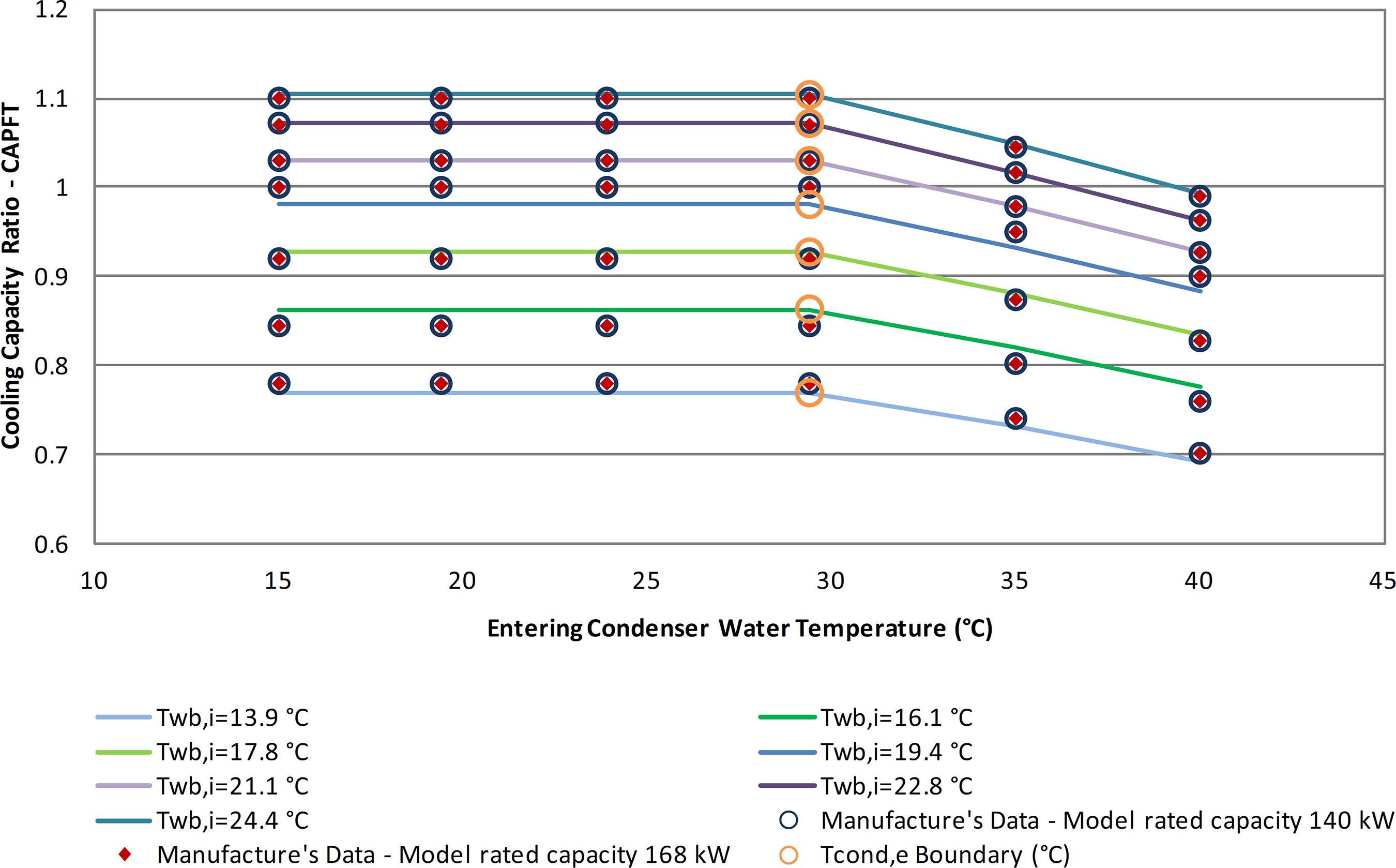
The curves CAPFT_low, CAPFT_high and T_cond,capft are presented in Figure 8 and the curves EIRFT_low, EIRFT_high and T_cond,EIRft are presented in Figure 9. These two figures show the difference between the correlations calculated from the regression coefficients and the values calculated directly from the data obtained from the catalog.

The curves T_cond,capft and T_cond,EIRft are considered to be the same. For all operating conditions, the limit temperature of T_cond,e is equal to 29.4ºC. Below this value the software uses the CAPFT_low and EIRFT_low curves and above this value it uses CAPFT_high and EIRFT_high.

The curves, and is evaluated in Figure 10. The power data as a function of PLR is determined by these curves and compared with the power data from the catalogs. The PLF curve is used for a PLR below 0.3.

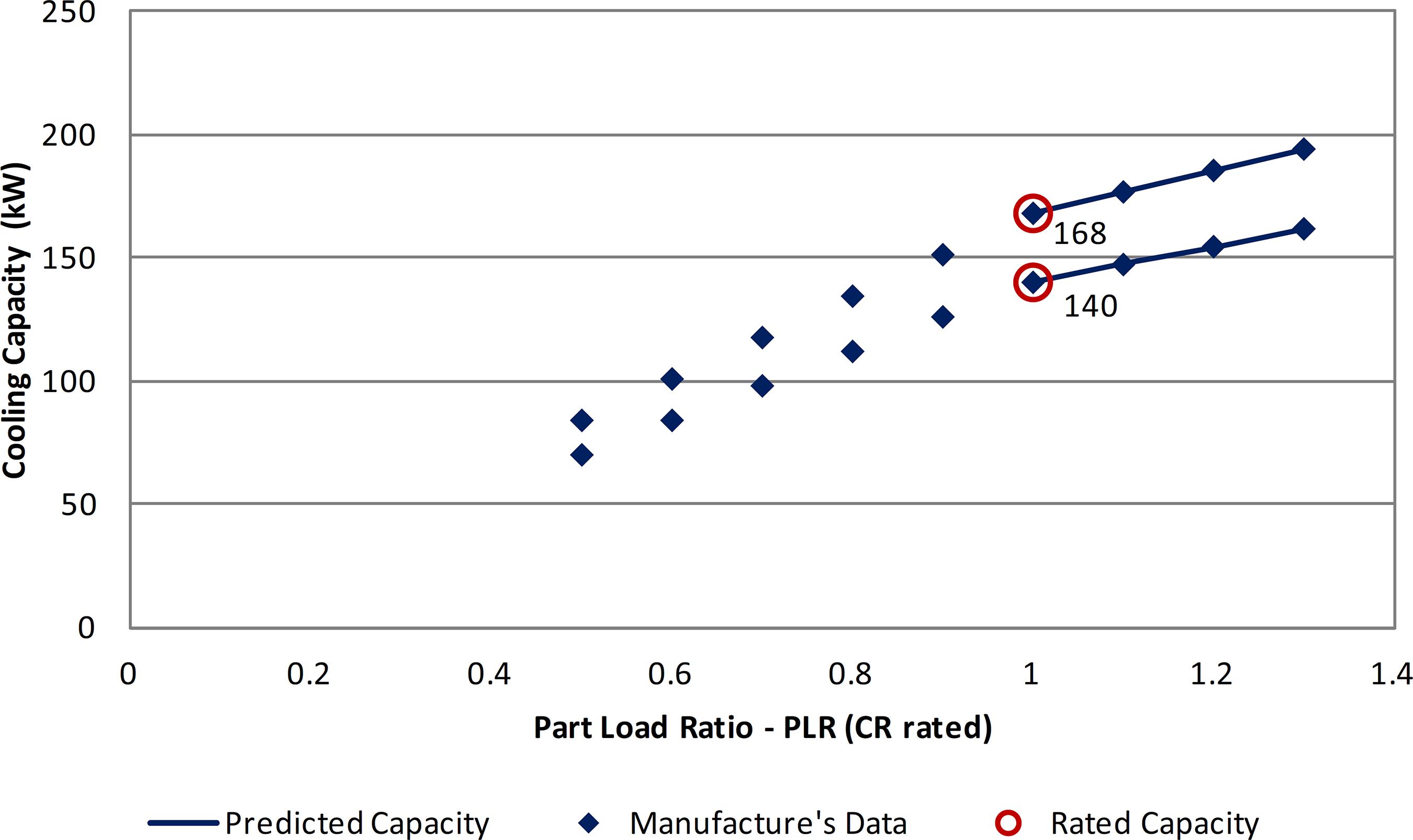
The available capacity as a function of PLR (equivalent to CR_rated) is calculated using the CR_correction curve and compared to the capacity data from the catalogs, as shown in Figure 11. The available capacity is not adjusted for PLR ≤ 1. The simulation model assumes that the capacity supplied is equal to the capacity required when the total capacity of the indoor units is less than or equal to the capacity of the outdoor unit. The manufacturer data for the P_correction are the same for the two outdoor units selected, as presented in Figure 12.

Figure 13 shows the performance of the COP in relation to the PLR. The results were calculated considering different ranges for an operation temperature. The value 5 presented in the Figure 13 represents the nominal COP, considering an internal wet-bulb temperature of 19.4 ºC and a condenser water temperature of 29.4 ºC. The simulated VRF outdoor unit shows a better performance in the PLR range of 40-60%. The efficiency is maximum at a PLR of 50% and decreases significantly until the minimum PLR of 30%.

Energy consumption according to end use

Figure 14 shows the annual energy consumption according to end use for the VAV and VRF air conditioning systems. For the constant schedule, the VRF system with CR > 1 provides energy consumption reductions of 17.8% and 11.7% in relation to the VAV systems with standard chillers and VSD chillers, respectively. For the variable schedule, the energy consumption reductions are 19.2% and 12.5% compared to the VAV systems with standard chillers and VSD chillers. The VRF system with CR > 1 provided reductions of 6.6% and 7.6% for the constant and variable building uses, respectively, when compared to the VRF system with CR < 1.

There is a decrease in the cooling energy consumption of the VAV and VRF systems for the variable schedule. The VAV systems showed a higher pump energy consumption when compared to VRF systems as the pump power system varies with cooling demand. The pump energy consumption of the VRF systems is set as constant. On the other hand, the fan energy consumption is higher for the VRF system when compared to VAV systems, for both schedules. The supply fan of the VRF indoor units operates continuously and the VAV supply fan varies the air flow rate according to the cooling demand.

Annual cooling efficiency analysis end-use

The cooling is the most influential end use energy based on a comparison of the energy consumption results obtained in this study (Figure 14). However, the pump and fan showed a significant influence on the annual energy consumption.

For both schedules, it was observed in Figure 14 that the annual energy consumption of the VAV systems was higher than that of the VRF systems. Even with a COP of 5 W/W under the nominal condition, the VRF systems consumed less cooling energy than the VAV systems with a nominal COP of 6.51 W/W (standard chillers) and 6.70 (VSD chillers). The COP values as a function of PLR showed that the VRF system performs better than the VAV with VSD chillers only in the PLR range of 40-55%. The VRF system with CR < 1 operates for a longer time with partial load than the VRF system with CR > 1, but the VRF system with CR < 1 resulted in inferior performance.

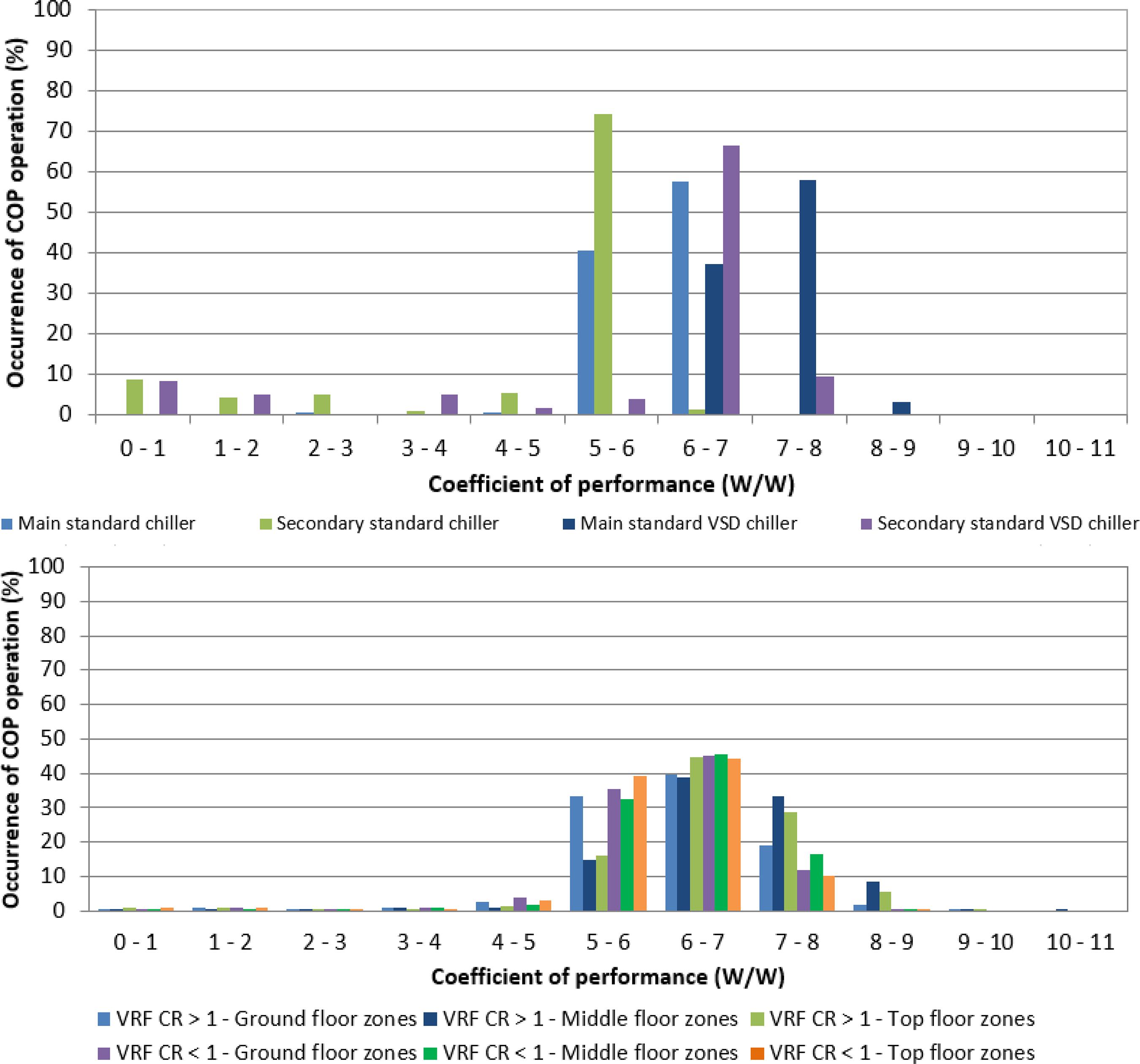
The results for the occurrence of COP operation for VAV and VRF systems, at constant and variable schedule is presented in Figure 15 and Figure 16, respectively.

Figure 15 shows that the VAV system with standard chillers presented the lowest COP values and that the operation of the secondary chiller contributed to reducing its performance in relation to the other systems. The main standard chiller operated with COP values from 6 to 7 for 87% of the time, and with COP values from 5 to 6 for 12% of the time. The secondary standard chiller operated in the COP range of 5 to 6 (76% of the time), with values of 6 to 7 occurring 5% of the time. The VAV system with VSD chillers presented higher COP values for the primary chiller, and lower COP values for the secondary chiller in relation to the values presented by the VRF system with CR <1. This resulted in the small difference in the cooling consumption results obtained for these systems.

For the VAV system with VSD chillers, COP ranges of 6 to 7 and 7 to 8 are predominant. The main and secondary chillers operated for 39% of the time in the former range. In the latter range, the main and secondary chillers operated for 45% and 23% of the time, respectively. It should also be noted that for a significant percentage of the time (16%) the main VSD chiller operated with COP values between 8 and 9. The COP ranges with the highest percentage of operation time for the VRF CR <1 system was 6 to 7 and 7 to 8. The VRF CR> 1 system presented the best COP values. The system operated most frequently with COP values in the ranges of 7 to 8, 6 to 7, and 8 to 9. It can be observed in Figure 16 that the COP values for the variable schedule are lower than those observed for the constant schedule, except for the main VSD chiller.

The COP values for the secondary chillers of the VAV systems contributed significantly to the reduction in the performance of these systems in relation to the VRF systems. For the VAV system with standard chillers, the main standard chiller operated with COP values of 6 to 7 for 58% of the time, and of 5 to 6 for 40% of the time. The secondary standard chiller operated mainly in the COP range of 5 to 6 (74% of the time). For the VSD chillers, the main chiller operated for 37% of the time and the secondary chiller for 66% of the time in the COP ranges of 6 to 7. In the COP ranges 7 to 8, the percentages of operation time were 58% and 9% for the main and secondary VSD chillers, respectively. The COP ranges in which the VRF CR>1 system operated most were 6 to 7, 7 to 8, and 5 to 6. For the VRF CR<1 system, the COP ranges that presented the highest percentages of operation time were 6 to 7, 5 to 6, and 7 to 8.

The annual COP values were intermediate, for both building schedules, based on the nominal COP for the VAV systems, ranging from 5 to 8. For the VRF systems, the annual COP values were higher than the nominal COP values, ranging from 5 to 9.

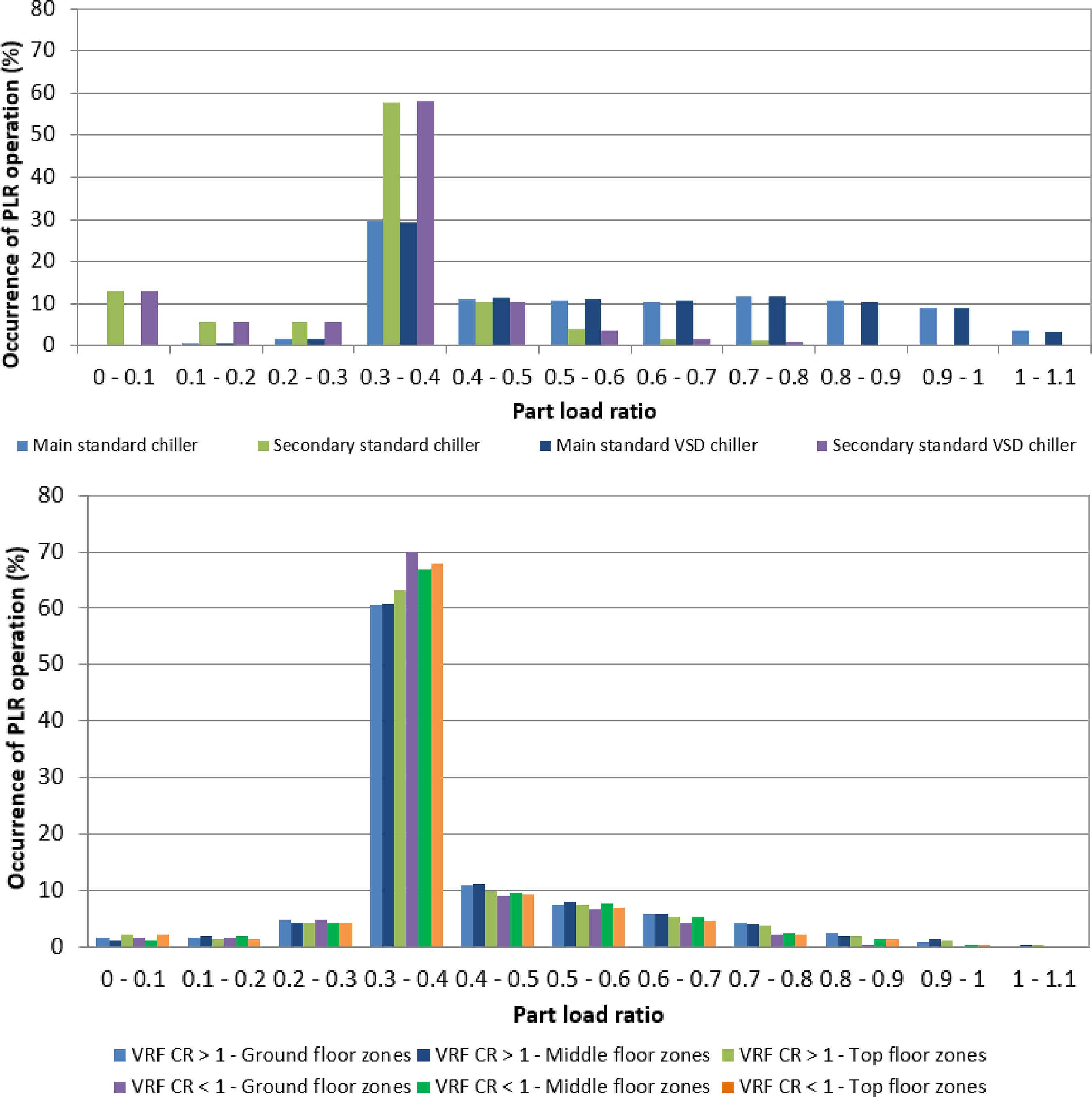
Figures 17 and 18 show the annual PLR results for the constant and variable building schedules, respectively. For the VAV systems, it was observed that the main chillers operated in the PLR range of 0.6 to 1.1 for 65% and 57% of the time for the constant and variable schedules, respectively. In this PLR range the main chiller presented a high efficiency. The secondary chillers operated for a significant amount of the time in the PLR range of 0.3 to 0.4 for both building use schedules (55% for the constant schedule and 58% for the variable schedule), but this PLR range was not associated with a high efficiency.

Moreover, the percentage of operation time at PLR values of < 0.3 increased from 18% to 26% with the use of the variable schedule. On the other hand, the VRF systems operated most of the time in the PLR range of 0.3 to 0.4, at which their performance starts to decrease. The percentages of operation time in this PLR range were 45% to 58% for the constant schedule and 60% to 70% for the variable schedule. In the PLR range of 0.4 to 0.7, at which the best performance was observed, the percentages of operation time were 38% and 23% for the constant and variable schedules, respectively.

Therefore, it can be noted that, in the case of the constant schedule, the air conditioning systems were operating at PLR values below the range considered to be the most efficient. Since the cooling demand is lower in the case of the variable schedule, the operation time spent in the less efficient PLR range for each air conditioning system increased, resulting the lower COP values.

The difference in the cooling energy consumption values for the VRF and VAV systems, for the variable schedule compared with the constant schedule, is mainly influenced by the partial load performance during the hottest period of the year. With a reduction in the PLR values, the VRF system operates for a higher percentage of the time at values closer to a PLR of 0.50. This PLR value is more competitively efficient, contributing to reducing the decrease in the annual performance of the VRF systems. In periods of milder outdoor temperatures, the performance characteristics are different. Although there is operation at a PLR of 0.50 during the period with the highest thermal load of the day, the PLR values are very low at the beginning and end of the day, hindering the cooling performance. In addition, the poor performance of the secondary chillers, due to the high percentage of operation time in PLR ranges associated with a significantly lower COP, contributes to the energy consumption difference observed.

For both building schedules, the higher cooling efficiency observed for the VRF CR > 1 system in relation to the VRF CR < 1 is due to the fact that the system operates at higher PLR values. The use of a larger outdoor unit aiming to increase the time of operation at partial load had a negative influence on the performance of the VRF air conditioning system evaluated in this study. Also, it can be noted that acceptable CR ranges vary from manufacturer to manufacturer. It is important to understand the reasons for the differences and if there are any advantages, disadvantages or risks to setting up a system with a larger or smaller CR.

For the VAV systems, the intermediate annual COP result of 5 to 8, compared to the nominal COP of 6.51 and 6.70, is associated with the balance between a satisfactory performance of the main chiller (PLR operation > 0.6) and very unsatisfactory performance for the secondary chiller (operation in PLR < 0.4). For VRF systems, the COP values of 5 to 9 compared to the nominal COP of 5 are associated with operation in the PLR range of 0.3 to 0.7.

Discussion

The performance of an air conditioning system is a function of its cooling capacity in response to the variation in the thermal loads throughout the year, and also many other factors, such as the ratio of the actual cooling loads to the design loads. This is particularly relevant to variable flow systems (either VAV or VRF). Therefore, the characteristics of the design and operation conditions should be considered to compare air conditioning systems, as well as climatic conditions, building materials and building use schedule.

This paper demonstrates the potential of building energy simulation (BES) to model different types of air conditioning systems. BES is becoming a key element to compare and analyze the energy performance of air conditioning systems (ZHOU et al., 2008ZHOU, Y. P. et al. Simulation and experimental validation of the variable-refrigerant-volume (VRV) air-conditioning system in EnergyPlus. Energy and Buildings , v. 40, p. 1041-1047, 2008.; RAUSTAD, 2013RAUSTAD, R. A variable refrigerant flow heat pump computer model in Energyplus, ASHRAE Transaction, v. 19, p. 299-308, 2013.; HONG et al., 2016HONG, T. et al. Development and validation of a new variable refrigerant flow system model in EnergyPlus. Energy and Building, v. 117, p. 399-411, 2016.). A comparison study between the simulation results of a VAV and VRF system is made to assess their cooling energy performance, particularly in partial load operation.

For VAV systems, for the same COP of 6.7 and PLR, the VSD chillers reached the best performance for all operating conditions. The final energy consumption was reduced by adopting chillers with better performance in partial loads. On the other hand, for both VAV systems, it was observed that dividing the nominal thermal load into two chillers was not very efficient. The operation of the secondary chiller significantly influenced the annual energy performance of the system by presenting a high frequency of COP values below the nominal COP.

For VRF systems, the hourly COP values were often higher than the nominal COP of 5, reducing the annual energy consumption. In this study, the VRF was more efficient in partial loads when compared to VSD chiller with nominal COP of 6.7. However, it was observed that the operation of the VRF systems was also not very efficient as the frequency of operation of these systems happened in a low PLR. Although this is a case study, these remarks are significant. The results show that the Brazilian regulation requirements related to air conditioning systems, such as the COP and IPLV, design and operation conditions, are not enough to obtain systems with adequate performance in terms of efficiency level and energy consumption. Measurement procedures considering part load operation and aligned with international standards need to be established in Brazil. Units of measurement and measurement procedures should be consistent to be possible to compare the energy performance of HVAC systems in different locations around the world.

The results reported in this paper address the importance in developing studies regarding VRF systems in Brazil in order to contribute with information that promotes the energy efficient use in buildings. The results show that the VRF systems presented less energy consumption when compared to the VAV systems. The same findings were observed in other studies (AYNUR; HWANG; RADERMACHER, 2009AYNUR, T. N.; HWANG, Y.; RADERMACHER, R. Simulation comparison of VAV and VRF air conditioning systems in an existing building for the cooling season. Energy and Buildings, v. 41, p. 1143-1150, 2009.; LIU, HONG, 2010LIU, X.; HONG, T. Comparison of energy efficiency between variable refrigerant flow systems and ground source heat pump systems. Energy and Buildings, v. 42, p. 584-589, 2010.; KIM et al., 2017KIM, D. et al. Evaluation of energy savings Potential of Variable Refrigerant flow (VRF) from Variable Air Volume (VAV) in the U.S. climate locations. Energy Reports, v. 3, p. 85-93, 2017.). However, it is important to note that this study is based on several assumptions and some of them are briefly discussed in this section.

Regarding building energy simulation, it is important to mention that system selection criteria may radically alter the findings. For example, a slight change in the performance curves used for each system would have a large effect on the results; or by using more efficient chillers. Some choices would likely make the VAV or VRF system a far more efficient choice (YIN; PATE; SWEENEY, 2016YIN, P.; PATE, M. B.; SWEENEY, J. F. Experimental performance evaluations and empirical model developments of residential furnace blowers with PSC and ECM motors. Journal of Building Engineering, v. 5, p. 239-248, 2016.). Building energy simulation results can contribute with information that promotes the energy efficient use in buildings. However, it is important to note that building energy simulation is based on several input data and machine performance has to be properly accounted.

There is only one investigated building, and the building requirements were established according to the Brazilian regulation for commercial buildings. Hence, the findings were primarily applicable to office buildings in Brazil.

It should be noted that other limitation is related to the assess for only one city in Brazil, Florianopolis. A difference in the annual air conditioning savings according to hot, mild and cold climates is presented by Kim et al. (2017)KIM, D. et al. Evaluation of energy savings Potential of Variable Refrigerant flow (VRF) from Variable Air Volume (VAV) in the U.S. climate locations. Energy Reports, v. 3, p. 85-93, 2017.. The VAV and VRF systems are expected to present different operation regarding climate condition.

One limitation of the simulation model is the lack of information on performance curves of each air conditioning system. The coefficients of the performance curves considered were obtained from the DataSet folder of the EnergyPlus program and from catalogs. In addition, it is important to mention that the advantages from VRF instead of VAV air conditioning system in this study is based on building energy simulation results. A detailed site survey, measurement and sub-metering can provide more comprehensive data for more detailed comparisons (YU et al., 2016YU, X. et al. Comparative study of the cooling energy performance of variable refrigerant flow systems and variable air volume systems in office buildings. Applied Energy, v. 183, p. 725-736, 2016.).

One important and recent initiative is the ASHRAE 205P - “Standard Representation of Performance Simulation Data for HVAC&R and Other Facility Equipment” (AMERICAN…, 2019AMERICAN SOCIETY OF HEATING, REFRIGERATING AND AIR-CONDITIONING ENGINEERS. ASHRAE 205P: standard representation of performance simulation data for HVAC&R and other facility equipment. Atlanta, 2019.). This standard it to facilitate equipment data exchange formats to improve the accuracy and efficiency of equipment modeling in simulation software. ASHRAE 205P will allow manufacturers and other data producers to implement data writing and reading methods supporting detailed performance data information such as capacity and input power for all operating conditions.

Conclusions

In this paper, the cooling energy performance of variable air volume (VAV) and variable refrigerant flow (VRF) were assessed and compared in terms of their cooling energy use. Based on the results the following conclusions can be drawn:

1. the performance curves of air conditioning equipment showed that the partial load operation characteristic of each system is as influential as the input data in the nominal condition for the annual energy consumption. The VRF systems, with COP of 5, presented lower energy consumption than the VAV systems, with COP of 6.7;

2. despite of achieving all requirements from the Brazilian regulation for office buildings regarding COP, IPLV and operating strategy, the VAV systems do not perform efficiently in partial loads;

3. for VRF systems, the only requirement of the Brazilian regulation is the nominal COP of 2.93, which is exceeded in this study. However, these systems do not perform well in partial load operation.

4. results indicate the need for the improvement of energy efficiency requirements for air conditioning systems in Brazil and highlight the importance of gaining information from the use of building energy simulation tools that allow air conditioning systems to be modelled. However, information regarding the air conditioning performance curves are essential to allow proper evaluation of its advantage when using building simulation for labeling or retrofit evaluation; and

5. the results address the importance in developing studies regarding VRF systems in Brazil in order to contribute with information that promotes the energy efficient use in buildings. Therefore, this comparative analysis with VRF and VAV systems, even with assumptions considered, contributes to other studies regarding design practices in Brazil.

Acknowledgements

The research reported in this paper was supported by The Brazilian Federal Agency for Support and Evaluation of Graduate Education - CAPES and the Brazilian National Council for Scientific and Technological Development - CNPq.

References

Publication Dates

History